The Design Choices Behind a Regime Detection Framework

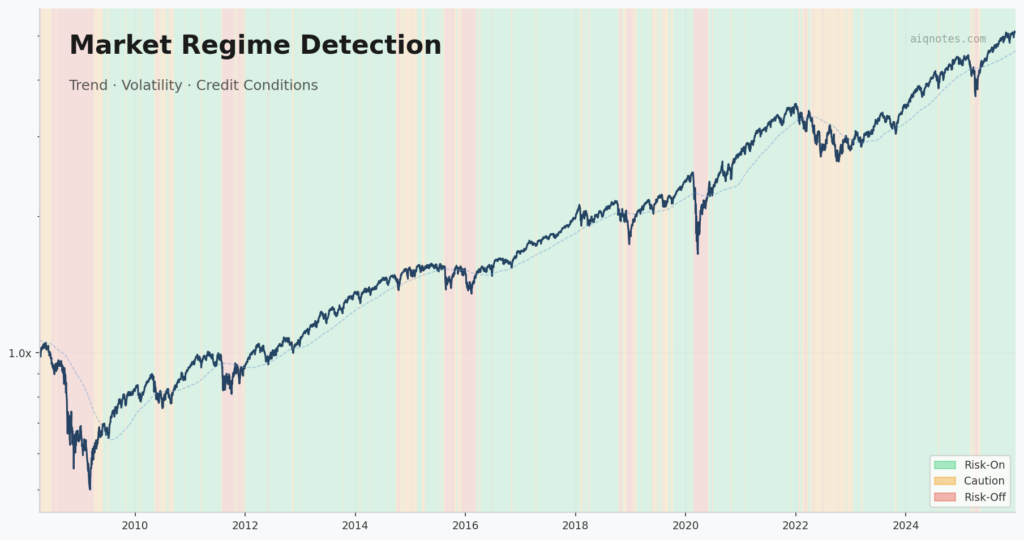
The article “Market Regime Identification Using Trend, Volatility, And Credit Conditions”, co-authored with my dear friend Fabio Baruffa, PhD, is published in the May 2026 issue of Technical Analysis of Stocks & Commodities (S&C V.44:05). It presents a framework that classifies market environments into three regimes — risk-on, caution, risk-off — using exactly three filters.

The article walks through the methodology and the backtest. This note picks up where the article leaves off — the design choices that don’t fit in a formal write-up. Why these three filters and not others. Why the regime table looks the way it does. Why nothing was optimized. The kind of decisions that shape a framework more than any formula.

This is also the first note published on AIQ Notes, the blog is born. The Python code behind the framework is available at the end (some EasyLanguage code included) — along with a way to stay in the loop for future research.

Three dimensions, one question

The framework answers one question: is the current market environment favorable for holding equity risk?

To answer it, the goal was to capture three separate dimensions of market stress. Not three versions of the same signal — three genuinely different perspectives.

Trend measures what the market is actually doing. Is price above or below its long-term average? This is the most basic, most robust signal in systematic trading. It’s slow, it’s late, and it works.

Volatility structure measures what the market expects to happen. Specifically, it compares short-term implied volatility (VIX) to 3-month implied volatility (VIX3M). When the ratio flips above 1.0 — the term structure goes into backwardation — the market is pricing in immediate stress. It’s a fear gauge, but a structural one.

Credit conditions measure what the bond market thinks of corporate risk. The ratio between high-yield bonds (HYG) and intermediate Treasuries (IEF) tracks the spread between “risky” and “safe” fixed income. When this Z-score drops sharply, credit markets are repricing default risk — often before equity markets fully react.

The point is that these three signals are conceptually independent. Trend is backward-looking (what happened). Volatility is forward-looking (what’s expected). Credit is cross-market (what bonds say about stocks). A framework built on three uncorrelated perspectives is more robust than one built on three variations of price momentum.

The design choices (and the ones not made)

Every filter involves design choices. Here’s what was picked and why.

SMA 200 for trend. Not 50, not 100, not an exponential average. The 200-day simple moving average is the most widely watched level in institutional trading. That’s not an accident — it captures roughly one trading year of data. But more importantly, the choice was deliberate: the SMA 200 is a convention, and conventions have value precisely because they’re shared. Choosing 200 is a conceptual decision, not an empirical one. Would 180 or 220 produce slightly different results? Probably. Would the difference survive out of sample? Doubtful.

VIX/VIX3M ratio with a threshold of 1.0. When short-term implied vol exceeds the 3-month measure, the term structure is inverted. The threshold isn’t arbitrary — it’s the mathematical definition of backwardation. No parameter fitting here; just reading a structural condition. This is the kind of choice worth favoring: driven by what the indicator means, not by what backtests best.

HYG/IEF Z-score with a threshold of −1.0. This one required more thought. The Z-score normalizes the HYG/IEF ratio against its own recent history (252-day lookback — one trading year). A threshold of −1.0 means the ratio is one standard deviation below its rolling mean. Is −1.0 better than −1.5 or −0.75? Probably not in a statistically meaningful way. But −1.0 is a reasonable “something unusual is happening” level. It triggers often enough to be useful, rarely enough to not cry wolf.

The regime table: common sense, not curve fitting

The three binary filters (on/off) create eight possible combinations. The regime classification maps them to three states:

• Risk-on: all three filters are clear. Full equity exposure.
• Risk-off: two or more filters are signaling stress. Exit equities entirely.
• Caution: exactly one filter is active. Reduce exposure (50%).

This table wasn’t optimized. It follows a simple principle: assume the market is fine unless evidence says otherwise, and weight the evidence by how many independent signals agree.

The asymmetry is deliberate. It takes multiple signals to go to risk-off (because the cost of being out of the market is high), but only one signal to move from risk-on to caution (because reducing exposure is a lighter response). The logic is: don’t overreact, but don’t ignore early warnings either.

One could argue that certain combinations deserve different treatment — say, that a credit signal alone should carry more weight than a trend signal alone. Maybe. But that’s where the line between structured reasoning and data mining gets blurry. The chosen rule can be explained in one sentence and doesn’t depend on which historical period is under examination. That matters more than squeezing another half-percent out of a backtest.

Why no optimization

This is the part that feels counterintuitive in a quantitative framework.

The filters use no fitted parameters. The SMA 200 is a convention. The VIX/VIX3M threshold is a structural definition. The credit Z-score uses a standard lookback and a round-number threshold. The regime table follows a symmetric voting logic.

It would have been straightforward to optimize everything. Run a grid search over SMA lengths from 50 to 300, test volatility thresholds from 0.85 to 1.15, sweep credit Z-score cutoffs, assign different weights to each filter. The backtest would look better. It always does.

The problem is well known: optimized systems are fragile. They fit the past precisely and the future poorly. Every parameter fitted is a degree of freedom spent, and in a framework with limited data (regime shifts happen a handful of times per decade), degrees of freedom run out fast.

By using conceptually motivated thresholds instead of empirically fitted ones, the framework trades a small amount of in-sample performance for a much better chance of working on data it hasn’t seen. This is a deliberate engineering choice, not a limitation. When someone says their system was “optimized on 20 years of data,” read: “overfit to 20 years of data.” The distinction is everything.

How much does each filter contribute?

A natural question: if the combined framework works, how much of that is each filter pulling its weight? To find out, here’s the same backtest run three times — once per filter, in isolation. Each single-filter strategy goes 100% invested when the filter is clear, 0% when it’s not.

	Ann. Return	Max Drawdown	Sharpe	Time Invested
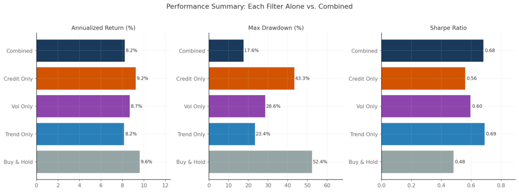
Buy & Hold	9.6%	−52.4%	0.48	100%
Trend Only	8.2%	−23.4%	0.69	76.5%
Volatility Only	8.7%	−28.6%	0.60	89.8%
Credit Only	9.2%	−43.3%	0.56	93.8%
Combined (3 filters)	8.2%	−17.6%	0.68	72% full + 19% half

A few things jump out.

The trend filter is the workhorse. Used alone, the SMA 200 produces the best Sharpe ratio (0.69) and the second-lowest drawdown (−23.4%). It’s out of the market about a quarter of the time, which is enough to dodge the worst of the major declines. This shouldn’t be surprising — trend following has decades of evidence behind it.

The volatility filter adds speed. Its drawdown is worse than trend alone (−28.6% vs −23.4%), and its Sharpe is lower (0.60). But the VIX/VIX3M ratio reacts faster than a 200-day moving average — it can signal stress weeks before the trend confirms it. Its value isn’t in standalone performance; it’s in catching the early stages of a selloff when the trend filter is still asleep.

The credit filter is the weakest standalone performer. A max drawdown of −43.3% means it missed most of the 2008 crisis on its own. The HYG/IEF Z-score only triggers in severe credit dislocations, which means it spends 93.8% of the time invested. That’s too little filtering to work as a standalone risk signal. But when it does trigger — 2008, March 2020 — it confirms that something genuinely systemic is happening.

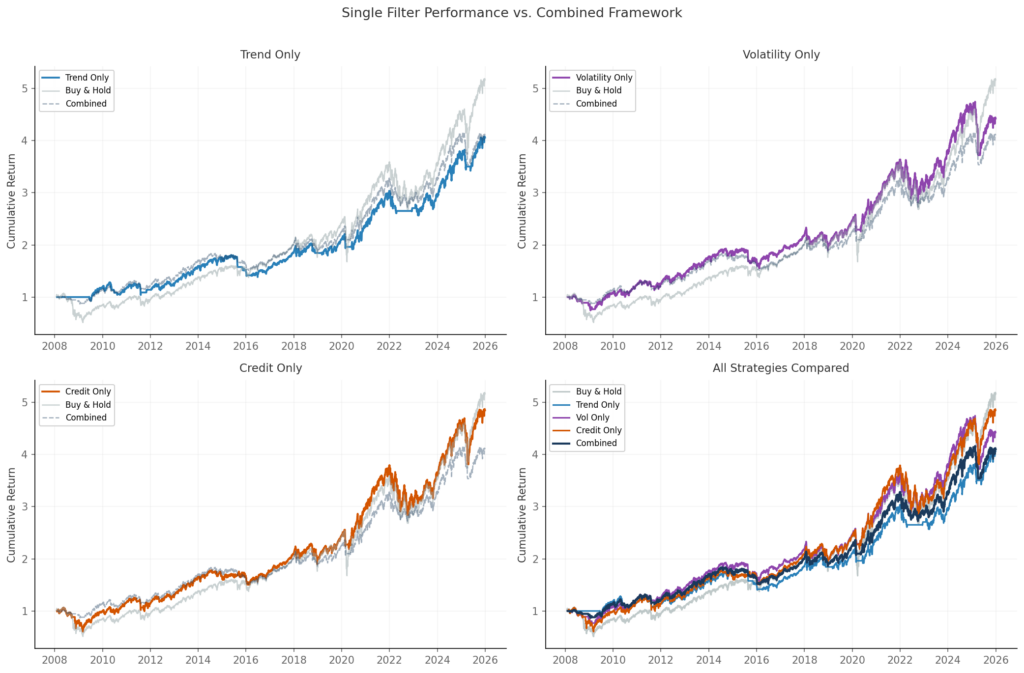
The cumulative return chart makes the pattern visible: each filter alone does something useful, but the combined framework draws a smoother line than any individual component. This is the diversification argument applied to signals rather than assets.

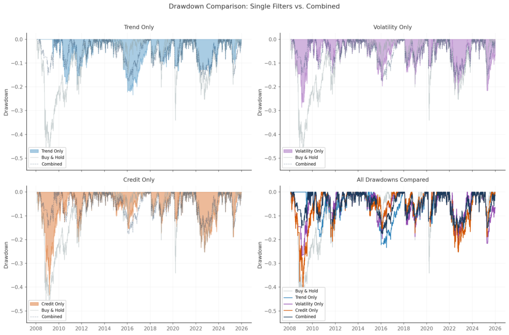
The drawdown comparison tells the most honest story. The combined framework’s worst drawdown (−17.6%) is substantially lower than any single filter’s worst case. No individual filter provides that level of protection — they need each other.

Is the combined framework “better” than trend-only? In terms of Sharpe ratio, it’s essentially the same (0.68 vs 0.69). In terms of maximum drawdown, the combined approach wins by 6 percentage points. Whether that difference justifies the added complexity of two extra filters is a legitimate question. For a quant who wants the simplest possible system, trend-only is a defensible choice. For someone who wants the best drawdown protection, the three-filter combination earns its place.

What the combined numbers show

For reference, here are the headline results from the full framework backtest (2006–2025, S&P 500):

	Buy & Hold	Regime Framework
Annualized Return	9.6%	8.2%
Maximum Drawdown	−52.4%	−17.6%
Sharpe Ratio	0.48	0.68
Regime Distribution	—	Risk-on 72%, Caution 19%, Risk-off 9%

The framework gives up about 1.4 percentage points of annual return and eliminates more than two-thirds of the worst drawdown. Is that a good trade? It depends entirely on objectives and risk tolerance. For someone who can stomach a −52% drawdown without flinching, buy-and-hold wins. For someone who can’t — and that’s most people, whether they admit it or not — a smoother ride at slightly lower return is worth a lot.

The regime distribution is also worth noting: the framework is invested at full capacity 72% of the time. It’s not an active timing system that trades in and out. It’s a risk filter that stays out of the way unless conditions deteriorate.

What could be done differently

Every design choice in this framework has alternatives worth exploring. The point of this section is not to suggest the current choices are wrong — the results above show they work. The point is to be transparent about what else is on the table, and to invite anyone with the code to test these ideas.

Trend filter alternatives. The SMA 200 is a convention, but it’s not the only option. A linear regression slope over the same window captures the direction of the trend rather than just the level, and may respond more smoothly to gradual shifts. An exponential moving average (EMA) gives more weight to recent prices, which can reduce lag — at the cost of more false signals in choppy markets. Dual moving average crossovers (e.g., SMA 50 / SMA 200) add a confirmation layer but introduce a second parameter to justify.

Volatility filter alternatives. The VIX/VIX3M ratio is a clean structural signal, but other measures of volatility stress exist. The VVIX (volatility of volatility) captures uncertainty about volatility itself. The VIX term structure slope across more maturities (VIX9D, VIX, VIX3M, VIX6M) could provide a richer picture. Realized vs. implied volatility ratios offer yet another angle — when implied is much higher than realized, the market is pricing in fear that hasn’t materialized yet.

Credit filter alternatives. The HYG/IEF ratio tracks high-yield vs. Treasury performance, but the choice of instruments matters. Using option-adjusted spreads (OAS) directly — available from FRED or ICE BofA indices — removes the duration component that pollutes ETF-based ratios. Investment-grade spreads (LQD/IEF) would capture a different tier of credit stress. TED spreads or LIBOR-OIS spreads offer a banking-sector perspective rather than a corporate one.

Regime table alternatives. The current table uses equal weighting — each filter has the same influence. A weighted approach, giving more importance to the trend filter (which performs best standalone) and less to credit (which performs worst), is a natural extension. But any weighting scheme introduces optimization, and the whole point of the current design is to avoid it. Another option: instead of binary on/off states, use continuous signals — for example, the distance between price and SMA 200, normalized as a Z-score. This turns the regime classification into a smooth function rather than a set of hard thresholds.

The optimization question. It would be straightforward to optimize the SMA length, the volatility threshold, the credit Z-score cutoff, and the regime weights. A walk-forward optimization with expanding windows could provide some out-of-sample validation. Whether the improvement survives transaction costs, data snooping bias, and the inevitable structural changes in markets is the real test.

None of these ideas are presented as improvements — they’re hypotheses. The code to test them is the same code that produced the results in this note. Run it, change the parameters, break it, rebuild it. That’s how research works.

What’s next

Future notes will pick up some of these threads: the SMA 200 vs. regression alternatives, sensitivity of the regime table to different voting rules, and possibly a fourth filter. Some will confirm the current design. Others won’t. Both are worth documenting.

---

---